|
|
FLOE Field Programs
Florida2000
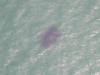
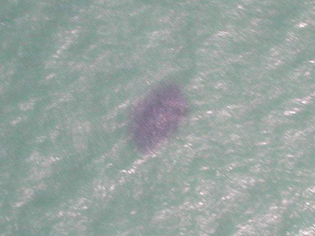
In December, 2000, the NOAA Fish Lidar
went to Tampa, Florida to look for schooling fish in the shallow waters
off the east coast of Florida. On the left is a photograph of a school
of mullet that was taken from the aircraft. We made several passes
over this school. The echo grams are two consecutive passes over
the same school from different directions. In the photograph, the
school looks darker than the surrounding water. The lidar clearly
shows the fish as a region of enhanced reflection.
In this experiment, the lidar measured a number of schools. A small boat
equipped with a scientific echosounder was directed to each school and made acoustic
measurements. In all, seven schools were captured both by the lidar and by the
echosounder. More schools were targeted by the lidar, but it proved impossible to get the
boat to most of these to obtain the acoustic measurements. The correlation between lidar
and acoustics for the seven schools was almost perfect (99.6%). There was also a
professional fish spotter on the plane with us. He was able to
identify the species of the
schools very reliably from the air.
James H. Churnside, David A. Demer, and Behzad Mahmoudi,
A comparison of lidar and echosounder measurements of fish, ICES Journal of Marine Science, 60: 147 154. 2003.
|
|
Alaska 2000
The NOAA lidar FLOE has flown along with a digital
camera in the waters off of southern Alaska in the summer of 2000.
This is program is funded by the North
Pacific Marine Research Initiative. The Principal Investigator
is Dr. Evelyn Brown of the Institute
of Marine Science of the University of Alaska at Fairbanks.
We evaluated airborne remote sensing, using lidar and color digital video, in the
North Pacific in 2000. Specific objectives were (1) to determine lidar depth-penetration
range, (2) to develop ocean color indices as a proxy for depth penetration and Chl a, (3)
to compare lidar with acoustic and net-sampling data, (4) to define diurnal variability
over large areas, and (5) to evaluate strengths and weaknesses. Depth penetration ranged
from 18 to 50 m in non-silty water, with lowest values observed inshore by day and
highest values on the continental shelf at night. A green index, derived from the three-
band video data, was significantly related to depth penetration and was in general
agreement with SeaWiFS satellite Chl a values. Significant correlations with acoustic
data were obtained in an area with a high concentration of capelin, Mallotus villosus.
Evelyn D. Brown, James H. Churnside, Richard L. Collins, Tim Veenstra, James J. Wilson, and Kevin Abnett,
Remote sensing of capelin and other biological features in the North Pacific using lidar and video technology, ICES Journal of Marine Science, 59: 000 000. 2002.
|
|
JUVESU 99
In August and September of 1999, the FLOE
flew on the Spanish Casa aircraft as part of the
European project on Experimental Surveys for the Assessment of Juveniles
(JUVESU). Flights
were made off of the northwest coast of Spain and in the Bay of Biscay.
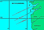
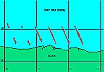
The map below shows the relative distribution of fish (in segments of about
1 nautical mile) off of the west coast of Spain seen during one evening
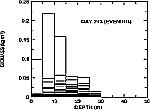
flight. The plot is a histogram of the depths of the fish densities.
These show a strong concentration of fish within the bay (Ria de Vigo)
that is mostly between 5 and 10 m. There is also a band of fish offshore
that is mostly between 5 and 25 m in depth.
|
|
|
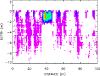
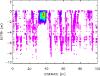
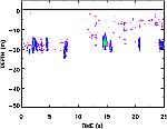
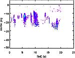
Typical "echogram" images are presented
below. The one on the left is about 1 nautical mile of data taken
offshore during midday of Julian day 243. Several small, dense schools
are seen. The other is an image taken in the evening of the same
day in the same area. The schools are larger, but more diffuse in
the evening than at midday. High-resolution images can be downloaded
by clicking on left image or right
image.
|
|
|
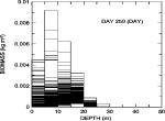
The map below is a typical map from the
Bay of Biscay. A larger area was flown on this day, and one can see
patches of fish distributed throughout the survey area. The depth
distribution shows a peak in the 5 - 10 m bin with fish detected down to
about 30 m.
|
|
California Squid 1999
In January 1999, ETL and the State
of California Department of Fish and Game conducted an experiment with
FLOE in California to see if we could detect squid. FLOE was reinstalled
on the King Air and
we flew around the southern California coast. The squid were plentiful
as were the squid fishermen.
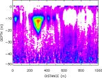
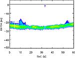
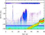
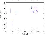
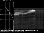
The following images are graphs of data. The X axis
is time in seconds and the Y axis is depth in meters. The laser fires 30
shots per second. There are 60 seconds worth of data plotted, so these
graphs represent 1800 shots from the laser. The aircraft we used was flying
at about 75 m/s (meters per second), so 60 seconds represents about 4.5
Km in distance. To learn more about FLOE's hardware, go to the
Instrument Page.
You may click on the image to see a slightly bigger
image(800x600) or if you click the link you will get a high resolution
image(2400x1800). The high resolution images will show the full detail
of the data and will print out very nice.
|
|
|
|
Image1 - 1/11/99, 21:49 PST, 34 degrees
3 minutes N, 119 degrees 0 minutes W.
The thick line at about 25 m is the bottom.
The lighter areas above the bottom at 10-15
and at 50-55 s are squid. For a high resolution
image,
click here.
|
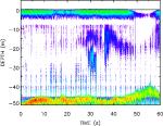
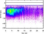
Image2 - 1/11/99, 21:07 PST, 33 degrees
55 minutes N, 119 degrees 59 minutes W.
There is a group of squid at 10 -12 s that is
a few m from the bottom. A much larger
group is at 30-35 s, and extends up to
10 m below the surface. For a high
resolution image,
click here.
|
|
|
|
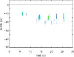
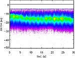
Image3 - 1/12/99, 19:47 PST, 33 degrees
54 minutes N, 119 degrees 58 minutes W.
The group here, at around 30 s, is clearly separated
from the bottom. The bottom just under the school
is at 50 m. For a high resolution image,
Click here.
|
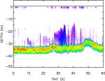
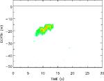
Image 4 - 1/12/99, 19:40 PST, 33 degrees
53 minutes N, 120 degrees 00 minutes W.
The main group here is at 30-33 s, and
extends from about 10 to 20
m above the
bottom. There is a second
group at
about 37 s that is just a little higher.
Above both groups is a plankton layer. For
a high resolution image, Click here.
|
|
JUVESU 98
In August and September of 1998, the FLOE
flew on the Spanish Casa aircraft as part of the
European project on Experimental Surveys for the Assessment of Juveniles
(JUVESU). Flights
were made off of the northwest coast of Spain, off of the west coast of
Portugal, and in the Bay of Biscay.
The "echogram" images below show typical
data from these flights. The first is an image of a number of small
schools of sardines in just off of the west coast of Galicia in Spain.
Time relates to distance by the aircraft speed, which was about 150 kts,
or 75 m/sec. The second image is of a much larger school off of the
west coast of Portugal. Clicking on the image brings up a larger
image on the screen. To see the full detail, click on small
schools or large school to bring
up the full resolution. This can be printed out with full resolution.
|
|
|
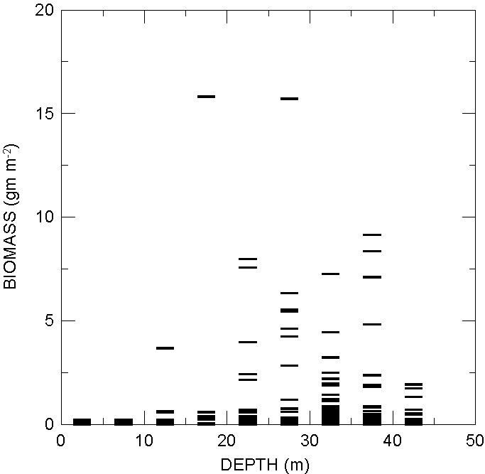
We can also obtain calibrated distributions
of fish in depth and by location. As an example, the following plot
shows the depth distribution for one particular flight. Each horizontal
line represents an integral over a 5-m depth bin and an average over 30
seconds of flight (about 2 km). We can see that the fish were
generally located between 20 and 40 m in depth.
|
|

|
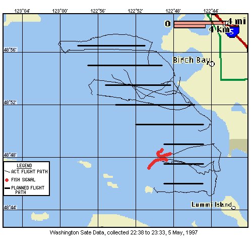
Washington State Herring Survey
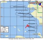
We found out that the Washington State Department
of Fish and Wildlife was going to do a herring survey in May, so we contacted
Norm Lemberg, Steve Burton and Mark Otoole and arranged to fly FLOE over
their survey operations. Later we would compare data to see how the different
survey methods worked.During the
day
and evening of May 5, 1997 we collected lidar data over the Puget Sound
off of the western coast of Washington State using FLOE in the Cessna.
In addition to the lidar there was an acoustic survey ship below that was
from the State of Washington Department
of Fish and Wildlife also mapping the area for herring. They would
chart the acoustic signal and if they detected fish, would trawl and sample
them. We overflew the same area and will compare the lidar data with the
acoustic data. Because the water of Puget Sound is so turbid, the lidar
can only see about 15 meters (50 feet) deep. In clear water we can usually
see to 40 meters (130 feet) deep. The trawl ship found the biggest concentration
of fish along the 48 degree North, 50.5 minute latitude track. The fish
were at between 22 to 27 fathoms (132 to 162 feet). Below is a map of the
transects that the ship traversed (Heavy Black Lines) and where we flew
(lighter black lines). The red spots over the black lines are where we
detected fish schools.
|
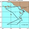
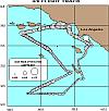
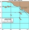
California 1997
Lidar Results
The maps below show some of the processed
data for the flight of April 6. The first map shows the flight track and
fish schools that were located along the track. The black line is our flight
track according to the Global Positioning System (GPS). The red squares
indicate fish schools. The second map shows the beam attenuation coefficient
of the lidar for the same flight track. Attenuation coefficient is a measure
of how clear the water is. Smaller spots indicate the water is more clear
and bigger spots indicate the water is less clear. The third map is a plot
of the ship track of the David Starr Jordan. The Jordan collected "egg
pump" data for the days of April 5 and 6. Egg pump data are where seawater
is pumped through a set of filters and then the fish eggs are counted.
In this case anchovy eggs were counted.
|
|
|
Here are some examples of the processed
data from these flights. In the following graphs, the Y axis is depth.
The 0 line is the ocean's surface. There is a blank section from the surface
to 5 meters deep. We don't look for fish in this region because of the
laser pulse reflection from the surface. The X axis is time. There are
30 shots of the laser in one second, so 30 seconds represents 900 laser
shots of data. In the data field, darker tint indicates a stronger return
signal. Click on any graph to get a larger more detailed graph (800x600).
If you want high resolution graphs that show all of the detail and are
suitable for publication, click on the High Resolution link below the graph.
These files are 2400x1800. They display much bigger than the screen, but
will print out very nicely and can be saved using the File and Save As
commands in your browser. Hit your back button to return.
|

|
|
|
In the first graph there are two distinct schools of fish
with the suggestion of a third. They range
from about
7-8 meters deep to about 22 to 23 meters
flight speed was about 75 meters per second.
(~140 Kts). The fish schools cover about
7 seconds
worth of data which gives total fish school
length of
about 525 meters. For a graph of 800x
600 click on
the picture. For a high resolution graph,
2400x1800,
click here.
|
The second graph shows a group of
dolphins. For a high resolution graph,
deep. Our
2400x1800, click here.
|
|
|
|
The third graph shows a school of anchovy.
For a high
resolution graph, 2400x1800, click here.
|
The fourth graph shows what a layer
of plankton looks like. For a high
resolution graph, 2400x1800,
click here.
|
|
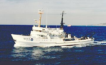
Fish Lidar Cruise '95
The 1995 cruise was conducted off of the Southern California
coast for three weeks during September 1995. The purpose of Cruise95 was
to collect FLOE (Fish Lidar, Oceanic, Experimental) data, acoustic data,
and in situ data from the water and then compare the performance
of FLOE with the acoustic instruments. Acoustic instruments have been
used for a number of years to detect fish schools.
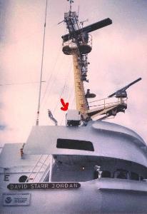
The picture at the left shows the David
Starr Jordan. At the right, the Fish Lidar optics package (arrow) is
shown mounted on the flying bridge.
If you would like to know more about the system hardware,
check out the Fish Lidar hardware page.
|
ECHOSOUNDER
|
LIDAR
|
|
|
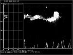
The picture on the right shows the sonar data for
one of the schools of fish seen from the ship. The picture on the left
is FLOE (lidar) data, collected at the same time. The vertical scales show
depth in meters, and both data sets were acquired in one minute. The white
blob on the right side of each picture is a school of fish. The left sides
of each picture are a single ping for the acoustic and a single laser pulse
from FLOE. It takes 600 laser pulses to give us one minute of data.
While the details are different because the
two instruments are not looking at exactly the same part of the school,
the general features are very similar.
|
|
|


